

Complicated prediction issues usually result in ensembles as a result of combining a number of fashions improves accuracy by lowering variance and capturing various patterns. Nonetheless, these ensembles are impractical in manufacturing as a consequence of latency constraints and operational complexity.
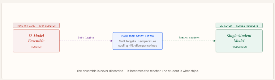
As a substitute of discarding them, Data Distillation presents a wiser method: preserve the ensemble as a instructor and practice a smaller scholar mannequin utilizing its comfortable likelihood outputs. This enables the coed to inherit a lot of the ensemble’s efficiency whereas being light-weight and quick sufficient for deployment.
On this article, we construct this pipeline from scratch — coaching a 12-model instructor ensemble, producing comfortable targets with temperature scaling, and distilling it right into a scholar that recovers 53.8% of the ensemble’s accuracy edge at 160× the compression.
What’s Data Distillation?
Data distillation is a mannequin compression approach by which a big, pre-trained “instructor” mannequin transfers its discovered habits to a smaller “scholar” mannequin. As a substitute of coaching solely on ground-truth labels, the coed is educated to imitate the instructor’s predictions—capturing not simply last outputs however the richer patterns embedded in its likelihood distributions. This method permits the coed to approximate the efficiency of advanced fashions whereas remaining considerably smaller and quicker. Originating from early work on compressing massive ensemble fashions into single networks, data distillation is now broadly used throughout domains like NLP, speech, and pc imaginative and prescient, and has turn into particularly necessary in cutting down large generative AI fashions into environment friendly, deployable techniques.
Data Distillation: From Ensemble Trainer to Lean Pupil
Establishing the dependencies
pip set up torch scikit-learn numpyimport torch
import torch.nn as nn
import torch.nn.purposeful as F
from torch.utils.information import DataLoader, TensorDataset
from sklearn.datasets import make_classification
from sklearn.model_selection import train_test_split
from sklearn.preprocessing import StandardScaler
import numpy as nptorch.manual_seed(42)
np.random.seed(42)Creating the dataset
This block creates and prepares an artificial dataset for a binary classification job (like predicting whether or not a consumer clicks an advert). First, make_classification generates 5,000 samples with 20 options, of which some are informative and a few redundant to simulate real-world information complexity. The dataset is then cut up into coaching and testing units to judge mannequin efficiency on unseen information.
Subsequent, StandardScaler normalizes the options so that they have a constant scale, which helps neural networks practice extra effectively. The information is then transformed into PyTorch tensors so it may be utilized in mannequin coaching. Lastly, a DataLoader is created to feed the information in mini-batches (dimension 64) throughout coaching, bettering effectivity and enabling stochastic gradient descent.
X, y = make_classification(
    n_samples=5000, n_features=20, n_informative=10,
    n_redundant=5, random_state=42
)

X_train, X_test, y_train, y_test = train_test_split(
    X, y, test_size=0.2, random_state=42
)

scaler = StandardScaler()
X_train = scaler.fit_transform(X_train)
X_test  = scaler.rework(X_test)

# Convert to tensors
X_train_t = torch.tensor(X_train, dtype=torch.float32)
y_train_t  = torch.tensor(y_train, dtype=torch.lengthy)
X_test_t   = torch.tensor(X_test,  dtype=torch.float32)
y_test_t   = torch.tensor(y_test,  dtype=torch.lengthy)

train_loader = DataLoader(
    TensorDataset(X_train_t, y_train_t), batch_size=64, shuffle=True
)
Mannequin Structure
This part defines two neural community architectures: a TeacherModel and a StudentModel. The instructor represents one of many massive fashions within the ensemble—it has a number of layers, wider dimensions, and dropout for regularization, making it extremely expressive however computationally costly throughout inference.
The coed mannequin, however, is a smaller and extra environment friendly community with fewer layers and parameters. Its objective is to not match the instructor’s complexity, however to be taught its habits via distillation. Importantly, the coed nonetheless retains sufficient capability to approximate the instructor’s choice boundaries—too small, and it received’t be capable to seize the richer patterns discovered by the ensemble.
class TeacherModel(nn.Module):
    """Represents one heavy mannequin contained in the ensemble."""
    def __init__(self, input_dim=20, num_classes=2):
        tremendous().__init__()
        self.internet = nn.Sequential(
            nn.Linear(input_dim, 256), nn.ReLU(), nn.Dropout(0.3),
            nn.Linear(256, 128),       nn.ReLU(), nn.Dropout(0.3),
            nn.Linear(128, 64),        nn.ReLU(),
            nn.Linear(64, num_classes)
        )
    def ahead(self, x):
        return self.internet(x)


class StudentModel(nn.Module):
    """
    The lean manufacturing mannequin that learns from the ensemble.
    Two hidden layers -- sufficient capability to soak up distilled
    data, nonetheless ~30x smaller than the total ensemble.
    """
    def __init__(self, input_dim=20, num_classes=2):
        tremendous().__init__()
        self.internet = nn.Sequential(
            nn.Linear(input_dim, 64), nn.ReLU(),
            nn.Linear(64, 32),        nn.ReLU(),
            nn.Linear(32, num_classes)
        )
    def ahead(self, x):
        return self.internet(x)
Helpers
This part defines two utility features for coaching and analysis.
train_one_epoch handles one full go over the coaching information. It places the mannequin in coaching mode, iterates via mini-batches, computes the loss, performs backpropagation, and updates the mannequin weights utilizing the optimizer. It additionally tracks and returns the common loss throughout all batches to watch coaching progress.
consider is used to measure mannequin efficiency. It switches the mannequin to analysis mode (disabling dropout and gradients), makes predictions on the enter information, and computes the accuracy by evaluating predicted labels with true labels.
def train_one_epoch(mannequin, loader, optimizer, criterion):
    mannequin.practice()
    total_loss = 0
    for xb, yb in loader:
        optimizer.zero_grad()
        loss = criterion(mannequin(xb), yb)
        loss.backward()
        optimizer.step()
        total_loss += loss.merchandise()
    return total_loss / len(loader)


def consider(mannequin, X, y):
    mannequin.eval()
    with torch.no_grad():
        preds = mannequin(X).argmax(dim=1)
    return (preds == y).float().imply().merchandise()
Coaching the Ensemble
This part trains the instructor ensemble, which serves because the supply of information for distillation. As a substitute of a single mannequin, 12 instructor fashions are educated independently with completely different random initializations, permitting each to be taught barely completely different patterns from the information. This range is what makes ensembles highly effective.
Every instructor is educated for a number of epochs till convergence, and their particular person take a look at accuracies are printed. As soon as all fashions are educated, their predictions are mixed utilizing comfortable voting—by averaging their output logits reasonably than taking a easy majority vote. This produces a stronger, extra steady last prediction, supplying you with a high-performing ensemble that may act because the “instructor” within the subsequent step.
print("=" * 55)
print("STEP 1: Coaching the 12-model Trainer Ensemble")
print("        (this occurs offline, not in manufacturing)")
print("=" * 55)

NUM_TEACHERS = 12
lecturers = []

for i in vary(NUM_TEACHERS):
    torch.manual_seed(i)                           # completely different init per instructor
    mannequin = TeacherModel()
    optimizer = torch.optim.Adam(mannequin.parameters(), lr=1e-3)
    criterion = nn.CrossEntropyLoss()

    for epoch in vary(30):                        # practice till convergence
        train_one_epoch(mannequin, train_loader, optimizer, criterion)

    acc = consider(mannequin, X_test_t, y_test_t)
    print(f"  Trainer {i+1:02d} -> take a look at accuracy: {acc:.4f}")
    mannequin.eval()
    lecturers.append(mannequin)

# Tender voting: common logits throughout all lecturers (stronger than majority vote)
with torch.no_grad():
    avg_logits     = torch.stack([t(X_test_t) for t in teachers], dim=0).imply(dim=0)
    ensemble_preds = avg_logits.argmax(dim=1)
ensemble_acc = (ensemble_preds == y_test_t).float().imply().merchandise()
print(f"n  Ensemble (comfortable vote) accuracy: {ensemble_acc:.4f}")
Producing Tender Targets from the Ensemble
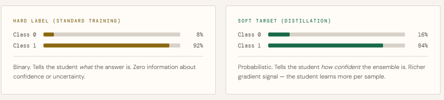
This step generates comfortable targets from the educated instructor ensemble, that are the important thing ingredient in data distillation. As a substitute of utilizing arduous labels (0 or 1), the ensemble’s averaged predictions are transformed into likelihood distributions, capturing how assured the mannequin is throughout all courses.
The perform first averages the logits from all lecturers (comfortable voting), then applies temperature scaling to easy the possibilities. The next temperature (like 3.0) makes the distribution softer, revealing refined relationships between courses that onerous labels can’t seize. These comfortable targets present richer studying alerts, permitting the coed mannequin to raised approximate the ensemble’s habits.
TEMPERATURE = 3.0   # controls how "comfortable" the instructor's output is

def get_ensemble_soft_targets(lecturers, X, T):
    """
    Common logits from all lecturers, then apply temperature scaling.
    Tender targets carry richer sign than arduous 0/1 labels.
    """
    with torch.no_grad():
        logits = torch.stack([t(X) for t in teachers], dim=0).imply(dim=0)
    return F.softmax(logits / T, dim=1)   # comfortable likelihood distribution

soft_targets = get_ensemble_soft_targets(lecturers, X_train_t, TEMPERATURE)

print(f"n  Pattern arduous label : {y_train_t[0].merchandise()}")
print(f"  Pattern comfortable goal: [{soft_targets[0,0]:.4f}, {soft_targets[0,1]:.4f}]")
print("  -> Tender goal carries confidence data, not simply class identification.")
Distillation: Coaching the Pupil
This part trains the coed mannequin utilizing data distillation, the place it learns from each the instructor ensemble and the true labels. A brand new dataloader is created that gives inputs together with arduous labels and comfortable targets collectively.
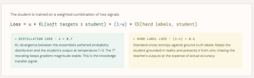
Throughout coaching, two losses are computed:
- Distillation loss (KL-divergence) encourages the coed to match the instructor’s softened likelihood distribution, transferring the ensemble’s “data.”
- Arduous label loss (cross-entropy) ensures the coed nonetheless aligns with the bottom fact.
These are mixed utilizing a weighting issue (ALPHA), the place a better worth provides extra significance to the instructor’s steerage. Temperature scaling is utilized once more to maintain consistency with the comfortable targets, and a rescaling issue ensures steady gradients. Over a number of epochs, the coed steadily learns to approximate the ensemble’s habits whereas remaining a lot smaller and environment friendly for deployment.
print("n" + "=" * 55)
print("STEP 2: Coaching the Pupil through Data Distillation")
print("        (this produces the only manufacturing mannequin)")
print("=" * 55)

ALPHA  = 0.7    # weight on distillation loss (0.7 = principally comfortable targets)
EPOCHS = 50

scholar    = StudentModel()
optimizer  = torch.optim.Adam(scholar.parameters(), lr=1e-3, weight_decay=1e-4)
ce_loss_fn = nn.CrossEntropyLoss()

# Dataloader that yields (inputs, arduous labels, comfortable targets) collectively
distill_loader = DataLoader(
    TensorDataset(X_train_t, y_train_t, soft_targets),
    batch_size=64, shuffle=True
)

for epoch in vary(EPOCHS):
    scholar.practice()
    epoch_loss = 0

    for xb, yb, soft_yb in distill_loader:
        optimizer.zero_grad()

        student_logits = scholar(xb)

        # (1) Distillation loss: match the instructor's comfortable distribution
        #     KL-divergence between scholar and instructor outputs at temperature T
        student_soft = F.log_softmax(student_logits / TEMPERATURE, dim=1)
        distill_loss = F.kl_div(student_soft, soft_yb, discount='batchmean')
        distill_loss *= TEMPERATURE ** 2   # rescale: retains gradient magnitude
                                           # steady throughout completely different T values

        # (2) Arduous label loss: additionally be taught from floor fact
        hard_loss = ce_loss_fn(student_logits, yb)

        # Mixed loss
        loss = ALPHA * distill_loss + (1 - ALPHA) * hard_loss
        loss.backward()
        optimizer.step()
        epoch_loss += loss.merchandise()

    if (epoch + 1) % 10 == 0:
        acc = consider(scholar, X_test_t, y_test_t)
        print(f"  Epoch {epoch+1:02d}/{EPOCHS}  loss: {epoch_loss/len(distill_loader):.4f}  "
              f"scholar accuracy: {acc:.4f}")
Pupil educated on on Arduous Labels solely
This part trains a baseline scholar mannequin with out data distillation, utilizing solely the bottom fact labels. The structure is an identical to the distilled scholar, making certain a good comparability.
The mannequin is educated in the usual means with cross-entropy loss, studying straight from arduous labels with none steerage from the instructor ensemble. After coaching, its accuracy is evaluated on the take a look at set.
This baseline acts as a reference level—permitting you to obviously measure how a lot efficiency achieve comes particularly from distillation, reasonably than simply the coed mannequin’s capability or coaching course of.
print("n" + "=" * 55)
print("BASELINE: Pupil educated on arduous labels solely (no distillation)")
print("=" * 55)

baseline_student = StudentModel()
b_optimizer = torch.optim.Adam(
    baseline_student.parameters(), lr=1e-3, weight_decay=1e-4
)

for epoch in vary(EPOCHS):
    train_one_epoch(baseline_student, train_loader, b_optimizer, ce_loss_fn)

baseline_acc = consider(baseline_student, X_test_t, y_test_t)
print(f"  Baseline scholar accuracy: {baseline_acc:.4f}")
Comparability
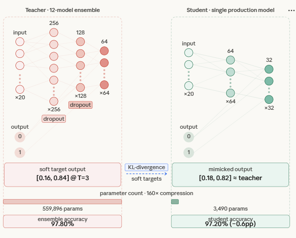
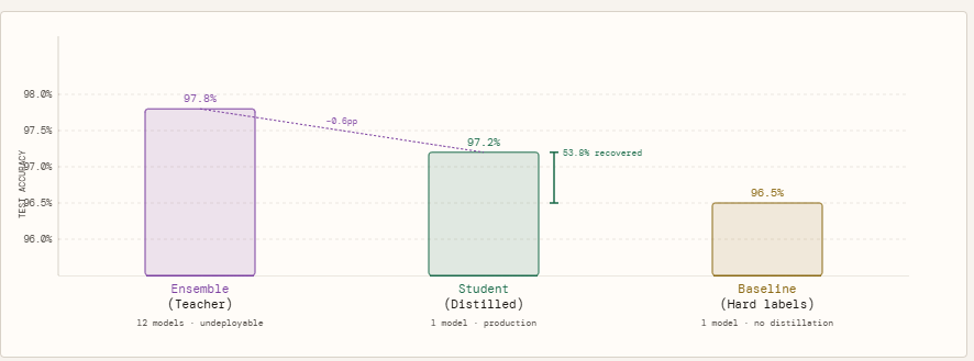
To measure how a lot the ensemble’s data really transfers, we run three fashions towards the identical held-out take a look at set. The ensemble — all 12 lecturers voting collectively through averaged logits — units the accuracy ceiling at 97.80%. That is the quantity we are attempting to approximate, not beat. The baseline scholar is the same single-model structure educated the standard means, on arduous labels solely: it sees every pattern as a binary 0 or 1, nothing extra. It lands at 96.50%. The distilled scholar is similar structure once more, however educated on the ensemble’s comfortable likelihood outputs at temperature T=3, with a mixed loss weighted 70% towards matching the instructor’s distribution and 30% towards floor fact labels. It reaches 97.20%.
The 0.70 proportion level hole between the baseline and the distilled scholar just isn’t a coincidence of random seed or coaching noise — it’s the measurable worth of the comfortable targets. The coed didn’t get extra information, a greater structure, or extra computation. It obtained a richer coaching sign, and that alone recovered 53.8% of the hole between what a small mannequin can be taught by itself and what the total ensemble is aware of. The remaining hole of 0.60 proportion factors between the distilled scholar and the ensemble is the sincere price of compression — the portion of the ensemble’s data {that a} 3,490-parameter mannequin merely can’t maintain, no matter how properly it’s educated.
distilled_acc = consider(scholar, X_test_t, y_test_t)

print("n" + "=" * 55)
print("RESULTS SUMMARY")
print("=" * 55)
print(f"  Ensemble  (12 fashions, production-undeployable) : {ensemble_acc:.4f}")
print(f"  Pupil   (distilled, production-ready)        : {distilled_acc:.4f}")
print(f"  Baseline  (scholar, arduous labels solely)          : {baseline_acc:.4f}")

hole      = ensemble_acc - distilled_acc
restoration = (distilled_acc - baseline_acc) / max(ensemble_acc - baseline_acc, 1e-9)
print(f"n  Accuracy hole vs ensemble       : {hole:.4f}")
print(f"  Data recovered vs baseline: {restoration*100:.1f}%")
def count_params(m):
return sum(p.numel() for p in m.parameters())
single_teacher_params = count_params(lecturers[0])
student_params = count_params(scholar)
print(f"n Single instructor parameters : {single_teacher_params:,}")
print(f" Full ensemble parameters : {single_teacher_params * NUM_TEACHERS:,}")
print(f" Pupil parameters : {student_params:,}")
print(f" Dimension discount : {single_teacher_params * NUM_TEACHERS / student_params:.0f}x")
Take a look at the Full Codes right here. Additionally, be happy to comply with us on Twitter and don’t overlook to hitch our 120k+ ML SubReddit and Subscribe to our E-newsletter. Wait! are you on telegram? now you’ll be able to be a part of us on telegram as properly.
Must accomplice with us for selling your GitHub Repo OR Hugging Face Web page OR Product Launch OR Webinar and many others.? Join with us

I’m a Civil Engineering Graduate (2022) from Jamia Millia Islamia, New Delhi, and I’ve a eager curiosity in Knowledge Science, particularly Neural Networks and their utility in numerous areas.